Parameter Estimation
Let us first import some libraries:
import numpy as np
%matplotlib inline
import matplotlib.pyplot as plt
from IPython.core.debugger import set_trace
np.random.seed(1234)
At the core of machine is model fitting or training, which is the process of estimating a parameter $\theta$ from our training set $\mathcal{D}$. There are many methods for producing such parameter estimates, which is denotes as $\hat{\theta}$, but most of it will boil dow to an optimization of the form:
$$\hat{\theta}=\arg\min_{\theta} \mathcal{L}(\theta)$$Where $\mathcal{L}(\theta)$ is some kind of loss function. What are these loss functions, and where do they come from? Well, they can come from either maximum likelihood methods, or Baysian methods.
To set the stage, consider the following simple case study: you are given observations of a series of coin flips from a possibly rigged/unfair coin. Based on this data we're given of the coin flips, we wish to figure out an estimate for the probability of the next conditional toss being a head (denote as 0) or tail (denote as 1). Of course, a coin flip scenario seems pretty random and contrived, but this coin flip problem can be generalized into much more useful binary processes (e.g if somebody is infected by a disease or not, a social media post being liked or not, or somebody purchasing a product or not).
Parameter Estimation
Suppose our coin toss outcome is probabilistically modelled by a Bernoulli distribution:
$$\text{Bernoulli}(x|\theta)=\theta^x(1-\theta)^{1-x}\;\;\;\;\;\;\;\;\text{or}\;\;\;\;\;\;\;\;\mathbb{P}(x|\theta)=\begin{cases} \theta & x=1 \\ 1-\theta & x=0\end{cases}$$We model the Bernoulli distribution as code in the following way, with a chosen value of $\theta$ being $0.4$ as the probability of obtaining heads:
#Function to compute parametric probability mass function
#If you pass arrays or broadcastable arrays it computes the elementwise bernoulli probability mass
Bernoulli = lambda theta,x: theta**x * (1-theta)**(1-x)
theta_star = .4
Bernoulli(theta_star, 1)
Recall a Bernoulli distribution is a discrete probability distribution that models a random variable that takes on a value of $1$ with probability $p$, and the value of $0$ with probability $q=1-p$. We also assume that our coin flips are i.i.d (independently and identically distributed). Independent as in the coin tosses have no memory, so the chance I get a certain result on one throw has no bearing on the chance I get the same result on the next throw (this would be true if the coin was fair). Identically in that the distrubution from which every throw was drawn from, so to speak, is and stays the same.
Our goal is to model the parameter $\theta$. Note that while the Bernoulli distribution only describes the outcome of a single coin toss trial, if we are interested in counting the total number of "successes" (or heads in our coin fliiping scenario) in a series of of multiple, independent Bernoulli trails (or coin tosses), we can use the Binomial distribution:
$$\text{Binomial}(N,N_h|\theta)={N\choose N_h}\theta^{N_h}(1-\theta)^{N-N_h}$$Where $N=|\mathcal{D}|$, the size of our training set, or rather the total number of coin tosses, and $N_h$ is the number of heads. As a reminder, the ${N\choose N_h}$ term are the binomial coefficients, which account for the number of sequence orderings we could observe as we count up the total number of heads/tails.
Maximum Likelihood
The most common approach to parameter estimation is to pick the parameters that assign the highest probability to the training data; this is called maximum likelihood estimation or MLE. The mathematical definition of the MLE is shown below:
$$\hat{\theta}_{\text{MLE}}\overset{\Delta}{=}{\arg}\max_{\theta}\mathbb{P}(\mathcal{D}|\theta)$$We made the assumption that our data are identically distributed. This means that they must have either the same probability mass function (if the data are discrete) or the same probability density function (if the data are continuous)
To simplify our conversation about parameter estimation, we are going to use the notation $p(x|\theta)$ to refer to this shared PMF or $f(x|\theta)$ for a PDF. Our new notation is interesting in two ways. First, we have now included a conditional on $\theta$ which is our way of indicating that the likelihood of different values of $X$ depends on the values of our parameters. Second, we are going to use the same symbol f for both discrete and continuous distributions.
Since we assumed each data point is independent, the likelihood of all our data is the product of the likelihood of each data point. Mathematically, the likelihood of our data given parameters $\theta$ is:
$$L(\theta)=\prod_{i=1}^n p(x_i|\theta)$$For our coin flip example, the likelihood function would be:
$$L(\theta;\mathcal{D})=\prod_{x\in \mathcal{D}}\text{Bernoulli}(x|\theta)$$In our code, we can plot the likelihood function for $n=10$ observations of a coin toss, resulting in the following
n = 10                                      #number of random samples you want to consider
xn = np.random.rand(n) < theta_star         #Generates n element boolean array where elements are True with probability theta_star and otherwise False
xn = xn.astype(int)                         #to change the boolean array to intergers [0:False, 1:True]
print("observation {}".format(xn))
#Function to compute the log likelihood
#Note that you can either pass this function a scalar(always broadcastable) theta or a broadcastable(in data axis) theta to get likelihood value or values
#Also note that we added an extra dimension in xn to broadcast it along theta dimension
L = lambda theta: np.prod(Bernoulli(theta, xn[None,:]), axis=-1)
#we generate 100 evenly placed values of theta from 0 to 1
theta_vals = np.linspace(0,1,100)[:, None]      #Note that we made the array broadcastable by adding an extra dimension for data
plt.plot(theta_vals, L(theta_vals), '-')
plt.xlabel(r"$\theta$")
plt.ylabel(r"Likelihood $L(\theta)$")
plt.show()
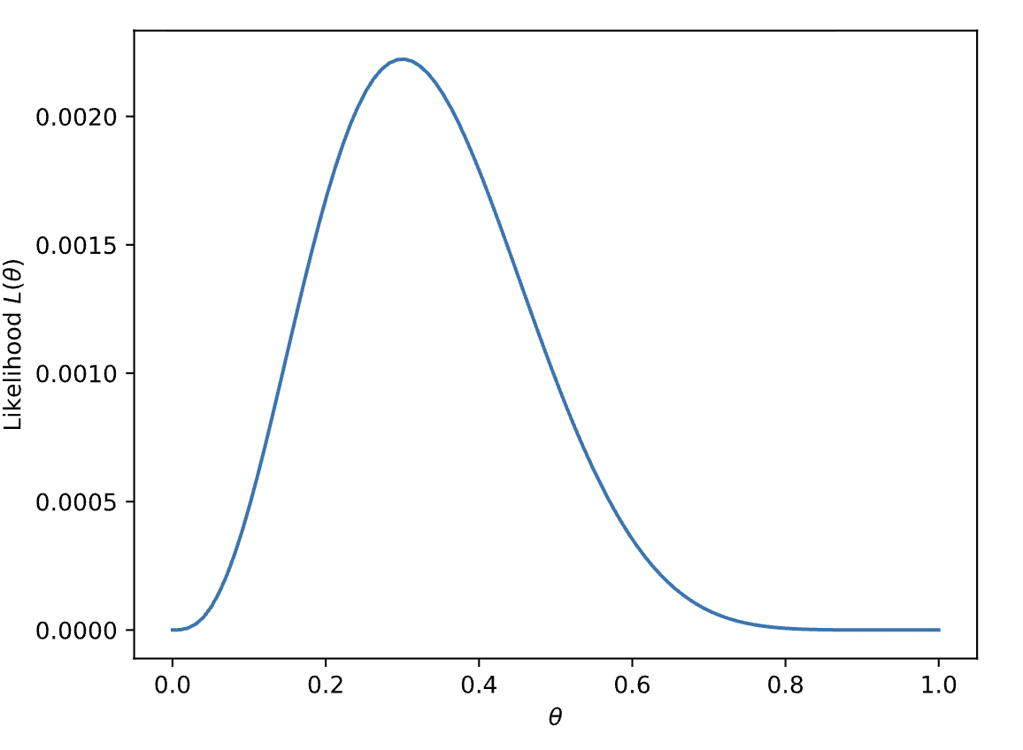
Something to notice with the likelihood function is that it tends towards extreme values for lots of observations, since taking the product of hundreds or thousands of data points sampled from distributions that lie between 0 and 1 will shrink the likelihood function into extremely small orders of magnitude, which will become inconvenient to work with on a computer. In addition, a cool property of arg max is that since log is a monotonic function, the arg max of a function is the same as the arg max of the log of the function! That’s nice because logs make the math simpler.
If we find the arg max of the log of likelihood, it will be equal to the arg max of the likelihood. Therefore, for MLE, we first write the log likelihood function:
$$\ell(\theta;\mathcal{D})=\log(L(\theta;\mathcal{D}))=\sum_{x\in \mathcal{D}}\log(p(x|\theta))$$So our problem to find the maximum likelihood parameter becomes:
$$\hat{\theta}_{\text{MLE}}={\arg}\max_{\theta}\ell(\mathcal{D};\theta)$$And of course, if we want to find the parameter $\theta$ that maximizes the log of the likelihood function, we take its derivative and set it equal to 0, and then solve for $\theta$. As a brief example, for the Bernoulli distribution, we would:
\begin{align*} \frac{\partial}{\partial\theta}\ell(\theta;\mathcal{D}) & = \frac{\partial}{\partial\theta} \sum_{x\in \mathcal{D}} \log\left(\theta^x(1-\theta)^{1-x}\right) \\ & = \frac{\partial}{\partial\theta}\sum_{x\in \mathcal{D}} \log\theta+(1-x)\log(1-\theta) \\ & = \sum_{x\in \mathcal{D}} \frac{x}{\theta}-\frac{1-x}{1-\theta} \end{align*}Setting equal to zero, and solving for $\theta$ gives:
$$\hat{\theta}_{\text{MLE}}=\frac{\sum_{x\in \mathcal{D}}x}{|\mathcal{D}|}$$Which is just the sample mean. In our coin toss scenario, this estimator would simply be the total number of heads observed, divided by the total number of coin flips.
The value of the likelihood shrinks exponentially as we increase the number of observations $N$. It is also customary to minimize the negative log-likelihood (NLL). Let's plot NLL for different $N$ - as we increase our data-points the MLE often gets better.
#Generates 2^12 element boolean array where elements are True with probability theta_star and otherwise False
xn_max = np.random.rand(2**12) < theta_star
for r in range(1,6):
    n = 4**r              #number of data samples for r-th iteration
    xn = xn_max[:n]       #slice them from the total samples generated
    #Function to compute the log likelihood (Implementation exactly similar to the likelihood function)
    ll = lambda theta: np.sum(np.log(Bernoulli(theta, xn[None,:])), axis=-1)
    theta_vals = np.linspace(.01,.99,100)[:, None]
    ll_vals = -ll(theta_vals)
    #Plot the log likelihood values
    plt.plot(theta_vals, ll_vals, label="n="+str(n))
    max_ind = np.argmin(ll_vals)                            #Stores the theta corresponding to minimum log likelihood
    plt.plot(theta_vals[max_ind], ll_vals[max_ind], '*')
#to get the horizontal line for theta
plt.plot([theta_star,theta_star], [0,ll_vals.max()], '--', label=r"$\theta^*$")
plt.xlabel(r"$\theta$")
plt.ylabel(r"Negative Log-Likelihood $-\ell(\theta)$")
plt.yscale("log")
plt.title("ML solution with increasing data")
plt.legend()
plt.show()
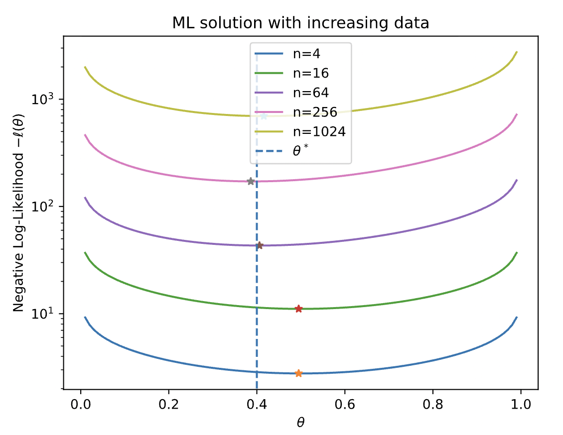
There are some drawbacks with this method of estimation, in particular, it's hard to gauge uncertainty in our estimators. Consider the following examples:
- For $\mathcal{D}=\{1\}$, $\hat{\theta}_{\text{MLE}}=1$. In our coin toss scenario, if we observe only one head, our estimator predicts all furture tosses will also be head! This doesn't seem right.
- For $\hat{\theta}_{\text{MLE}}=0.2$ for both experiments where we perform 5 trials and found success $1/5$ of the time, and also we perform 5000 trials and found success $1000/5000$ of the time. The MLE will be the same for each, but surely we should be confident in our estimator for the experiment where we performed 5000 trials.
Bayesian Approach
In our to capture the uncertainty in our estimated parameter, we use a Bayesian Inference approach, where we model uncertainty about parameters using a probability distribution (as opposed to just computing a point estimate). First, we define the following terms:
- Prior Distribution: $\color{blue} p(\theta)$ Here, our unknown parameter $\theta$ is viewed as a random variable with a probability distribution. This prior distribution is specified before any data are collected and provides a theoretical description of information about $\theta$ that was available before any data were obtained.
- Posterior Distribution: $\color{red} p(\theta|\mathcal{D})$ Here, this is an "updated" conditional distribution of our parameter $\theta$ conditioned on our observed training $\mathcal{D}$. The posterior distribution summarizes all of the pertinent information about the parameter $\theta$ by making use of the information contained in the prior for θ and the information in the data.
- Likelihood: $\color{green}p(\mathcal{D}|\theta)$ As a function of the data with our parameter fixed, this indicates the compatibility of the data $\mathcal{D}$ with the given paramter known $\theta$. In essence, it reflects the data we expect to see for each setting of the parameters.
- Marginal Likelihood: $\color{purple}p(\mathcal{D})$ Marginal since it is computed by marginalizing over (or integrating out) the unknown $\theta$. This can be interpreted as the average probability of the data, where the average is wrt the prior. Note, however, that $p(\mathcal{D})$ is a constant, independent of $\theta$, so we will often ignore it when we just want to infer the relative probabilities of $\theta$ values.
And then, we update our degree of certainty given our data using Bayes' Rule:
$$\color{red}p(\theta|\mathcal{D})\color{black}=\frac{\color{blue} p(\theta)\color{green}p(\mathcal{D}|\theta)}{\color{purple}p(\mathcal{D})}=\frac{\color{blue} p(\theta)\color{green}p(\mathcal{D}|\theta)}{\color{purple}\int p(\theta')p(\mathcal{D}|\theta')d\theta'}$$Notice from the above equation we can get a single point estimate for $\theta$ by collapsing the posterior distritbuion into one point - either by taking the maximum value, the mean of the distribution, the mode, etc.
In our coss toss example, we can form our likelihood as before using the iid assumption:
$$\color{green} p(\mathcal{D}|\theta)=\prod_{c\in \mathcal{D}}\text{Bernoulli}(x;\theta)=\theta^{N_h}(1-\theta)^{N_t}$$How should we handle the prior distribution $\color{blue}p(\theta)$? To simplify computations, we will assume that the prior is a conjugate prior for the likelihood function, meaning that the postierior is in the same parametrized family as the prior. To ensure this property when using the Bernoulli (or Binomial) likelihood, we should use a prior of the following form:
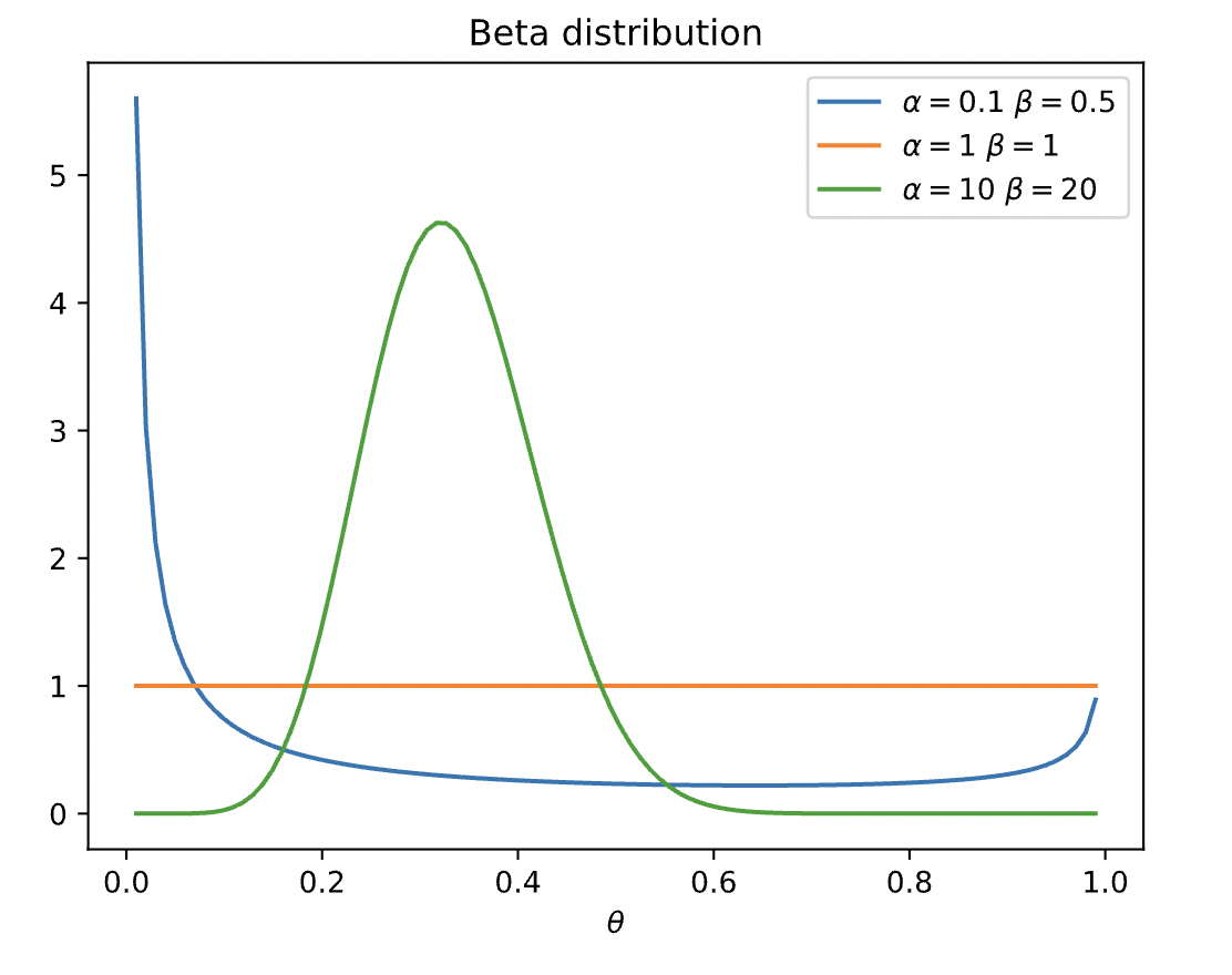
$$p(\theta|a,b)\propto \theta^a(1-\theta)^b$$We recognize this as the pdf of a Beta distribution. Recall the full density is:
$$\text{Beta}(\theta|\alpha, \beta)=\frac{\Gamma(\alpha+\beta)}{\Gamma(\alpha)\Gamma(\beta)}\theta^{\alpha-1}(1-\theta)^{\beta-1}$$Where the factor outside is a normalization constant. Recall the Gamma function $\Gamma(\alpha+1)=\alpha\Gamma(\alpha)$ is a generalization of factorial for the real numbers. Plotting the Beta distribution for different values of $\alpha, \beta>0:$
from scipy.special import beta                                      #we import beta function from scipy
#Function to compute probability density function of beta distribution parameterized by a and b
Beta = lambda theta,a,b: ((theta**(a-1))*((1-theta)**(b-1)))/beta(a,b)
#Plot the distribution for different values of a and b
for a,b in [(.1,.5), (1,1), (10,20)]:
    theta_vals = np.linspace(.01,.99,100)
    p_vals = Beta(theta_vals, a, b)
    plt.plot(theta_vals, p_vals, label=r"$\alpha=$"+str(a)+r" $\beta=$"+str(b))
plt.xlabel(r"$\theta$")
plt.title("Beta distribution")
plt.legend()
plt.show()
So we set our prior to be:
$$\color{blue}p(\theta)\propto \theta^{\alpha-1}(1-\theta)^{\beta-1}$$For the posterior, $\color{red} p(\theta|\mathcal{D})$, we multiply the Bernoulli likelihood equation with the Beta prior, in the end obtaining a Beta posterior with parameters $\alpha+N_h$, and $\beta+N_t$:
$$\color{red}p(\theta|\mathcal{D})\propto \theta^{\alpha+N_h-1}(1-\theta)^{\beta+N_t-1}$$Note that the parameters of the prior, $\alpha,\beta$, are known as pseudo counts, or preliminary guesses for the frequency of observations, that are ultimately corrected by the posterior. As you can see, this solves our issue that we had with MLE, in that it will scale and "correct" more aggressively the more observations we make. That is, with a small number of observations, the prior will dominate, but as we increase the number of observations $N=|\mathcal{D}|$, the effect of the prior diminishes and the likelihood term will dominate the posterior.
Let's confirm this with code:
ax = np.random.rand(2**12) < theta_star
a0, b0 = 10, 10
theta_vals = np.linspace(.01,.99,1000)[:, None]
posterior = Beta(theta_vals, a0, b0)              #get the prior distribution
plt.plot(theta_vals, posterior , label="prior")
for r in range(1,6):
    n = 4**r
    xn = xn_max[:n]
    nh = np.sum(xn)                                           #number of heads out of n data samples
    posterior = Beta(theta_vals, a0+nh, b0+n-nh)              #update the posterior based on the number of samples
    plt.plot(theta_vals, posterior , label="n="+str(n))

plt.plot([theta_star,theta_star], [0,posterior.max()], '--', label=r"$\theta^*$")
plt.xlabel(r"$\theta$")
plt.ylabel(r"Posterior")
plt.title("Posterior dist. with increasing data")
plt.legend()
plt.show()
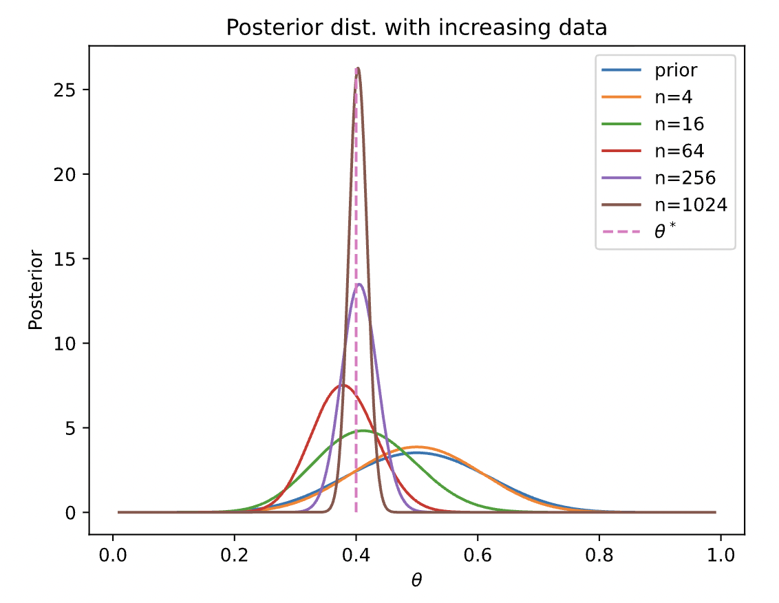
Note that the posterior becomes more peaked around $\theta=0.4$, while also reflecting our uncertainty in the mode (note the decrease in variance).
Posterior Predictive
Suppose we want to predict future observations. A very common approach is to first compute an estimate of the parameters based on training data, $\hat{\theta}(\mathcal{D})$ and then to plug that parameter back into the model and use $p(y|\hat{\theta})$ to predict the future. However, this can result in overfitting. As an extreme example, suppose we have seen $N=3$ heads in a row. The MLE is $\hat{\theta} = 3/3 = 1$. However, if we use this estimate, we would predict that tails are impossible.
Instead, to make predications, we can calculate the average prediction over all possible values of $\theta$, (marginalizaing it out) and for each $\theta$, we weight the prediction by the posterior probability of that parameter being true, i.e computer
$$p(x|\mathcal{D})=\int_{\theta}\color{red}p(\theta|\mathcal{D})\color{blue}p(x|\theta)\color{black}d\theta$$How can we use this in our coin flip scenario? Well, starting from our Beta prior $\color{blue}p(\theta)=\text{Beta}(\theta|\alpha, \beta)$, we then observe $N_h$ heads and $N_t$ tails, and we compute our posterior to be $\color{red}p(\theta|\mathcal{D})=\text{Beta}(\theta|\alpha+N_h,\beta+N_t)$, then we compute the probability of observing heads $(x=1)$ using our posterior predictive distribution:
\begin{align*}p(x=1|\mathcal{D}) & = \int_{\theta}\text{Bernoulli}(x=1|\theta)\text{Beta}(\theta|\alpha+N_h,\beta+N_t)d\theta \\ & = \int_{\theta}\theta \text{Beta}(\theta|\alpha+N_h,\beta+N_t)d\theta \\ & = \frac{\alpha+N_h}{\alpha+\beta+N} \end{align*}Which is just the mean of a Beta distribution with parameters $\alpha+N_h$ and $\beta+N_t$.
Compare this with the above example of observing three heads. The MLE estimate was $\hat{\theta} = 3/3 = 1$, meaning we should observe heads 100% of the time. but now if we take $\alpha=\beta=10$, with the posterior prediction method, we obtain the probability of observing heads as $(10+3)/(10+10+3)=13/23$.
A special case is if we use a uniform distribution for the prior, the posterior predictive becomes:
$$p(x=1|\mathcal{D})=\frac{N_h+1}{N+2}$$This is known as Laplace smoothing or Laplace’s rule of succession .
Maximum a Posteriori (MAP)
In many applications calculating the posterior distribution is not easy. A cheap alternative is to calculate the mode (maximum) of the posterior distribution:
$$\hat{\theta}_{\text{MAP}}=\arg\max_{\theta}p(\theta|\mathcal{D})=\arg\max_{\theta}p(\theta)p(\mathcal{D}|\theta)$$And similar to MLE, it also suffices to find the maximum of the log of the posterior, i.e
$$\hat{\theta}_{\text{MAP}}=\arg\max_{\theta}\log\;p(\theta)+\log\;p(\mathcal{D}|\theta)$$For our coin toss example, maximizing our posterior $p(\theta|\mathcal{D})=\text{Beta}(\theta|\alpha+N_h,\beta+N_t)$ gives us:
$$\hat{\theta}_{\text{MAP}}=\frac{\alpha+N_h-1}{\alpha+\beta+N_h+N_t-2}$$